Building evals for LLM-powered applications is hard. One could spend weeks or months and still not have evals that correlate well with application-specific performance. To make matters worse, improved performance on generic benchmarks, such as MMLU or MT-Bench, doesn’t always translate to improved performance on our tasks. (View Highlight)
This is my attempt to reduce the time we spend evaluating evals so we have more time evaluating application and task performance. We’ll focus on automated evals for the more common, simpler tasks of classification, summarization, and translation. We’ll also see how to evaluate the risk of copyright regurgitation and toxicity. For each, we’ll discuss how to compute and quantify them via key metrics. (View Highlight)
• Classification: Recall, precision, ROC-AUC, PR-AUC, separation of distributions
• Summarization: Factual consistency, relevance, length adherence
• Translation: Quality measures via statistical and learned metrics
• Copyright: Exact regurgitation, near-exact reproduction
• Toxicity: Proportion of toxic generations on regular and toxic prompts (View Highlight)
While these tasks are relatively simple and LLMs likely perform well on them, we’ll still want to have solid evals. For example, Voiceflow’s eval harness for intent classification helped them catch a 10% performance drop when upgrading from the deprecating gpt-3.5-turbo-0301 to the more recent gpt-3.5-turbo-1106. (View Highlight)
We can apply LLMs for classification by providing a document and prompting the LLM to predict the sentiment or topic, or to check for abusive content or spam. The expected output can be a categorical label (“positive”) or the probability of the label (“0.1”). Similarly, LLMs can extract information from a document by prompting it to return JSON with keys for desired attributes such as “names” and “dates”. (View Highlight)
For categorical outputs, we can compute aggregate statistics such as recall, precision, false positives/negatives, etc. This also applies to extraction: What proportion of ground truth attributes were extracted (recall)? What proportion of extracted attributes were correct (precision)? IMHO, accuracy is too crude a metric to be useful. The Wikipedia page is a good reference for these metrics. In a nutshell:
• Recall: Proportion of true positives that were correctly identified. If there were 100 positive instances in our data and the model identified 80, recall = 0.8
• Precision: Proportion of the model’s positive predictions that were correct. If the model predicted positive 50 times but only 30 were truly positive, precision = 0.6
• False positive: Model predicted positive but actually negative
• False negative: Model predicted negative but actually positive (View Highlight)
It gets interesting when our models can output probabilities instead of simply categorical labels (e.g., language classifiers, reward models). Now we can evaluate performance across different probability thresholds, using metrics such as ROC-AUC and PR-AUC. (View Highlight)
The Receiver Operating Characteristic (ROC) curve plots the true positive rate against the false positive rate at various thresholds, visualizing the performance of a classification model across all classification thresholds. The ROC Area Under the Curve (ROC-AUC) is an aggregate measure of performance that ranges from 0.0 to 1.0. A model that’s no better than a coin flip would have ROC-AUC = 0.5 while a model that’s always correct has ROC-AUC = 1.0. (Cramer would have ROC-AUC < 0.5.) (View Highlight)
ROC-AUC has some nice properties. First, it’s robust to class imbalance because it specifically measures true and false positive rate. In addition, it doesn’t require picking a threshold since it evaluates performance across all thresholds. Finally, it is scale-invariant, thus it doesn’t matter if your model’s predictions are skewed. (View Highlight)
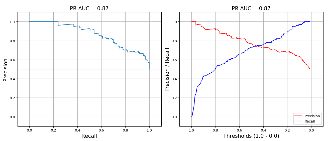
The Precision-Recall curve plots the trade-off between precision and recall across all thresholds. As we update the threshold for positive predictions, precision and recall change in opposite directions. A higher threshold leads to higher precision (fewer false positives) but lower recall (more false negatives), and vice versa. The area under this curve, PR-AUC, summarizes performance across all thresholds. Like ROC-AUC, a perfect classifier has PR-AUC = 1.0 while a random classifier has PR-AUC = 0.0. (View Highlight)
PR curves with PR-AUC = 0.87
The standard PR curve (left below) plots precision and recall on the same line, starting from the top-right corner (high precision, low recall) and moving towards the bottom-left corner (low precision, high recall). I prefer a variant (right below) where precision and recall are plotted as separate lines—this makes it easier to understand the trade-off between precision and recall since they’re both on the y-axis. (View Highlight)
Another useful diagnostic is plotting the distribution of predicted probabilities for each class. This visualizes how well the model is separating the classes. Ideally, we’d see two distinct peaks at 0.0 for the negative class and 1.0 for the positive class. This suggests that the model is confident in its predictions and can cleanly separate the classes. On the other hand, if there’s significant overlap between the distributions, it suggests that it may be difficult to pick a threshold to use in production.
Separation of distributions with JS divergence = 11.078 (View Highlight)
To quantify the separation of distributions, we can compute the Jensen-Shannon divergence (JSD), a symmetric form of Kullback-Leibler (KL) divergence. Concretely, we compute the average of KL divergence from (i) distribution P to the average of P and Q (M) and (ii) from distribution Q to the average of P and Q (M). Nonetheless, I’ve found JSD hard to interpret and prefer to look at the graph directly. (View Highlight)
Examining the separation of distributions is valuable because a model can have high ROC-AUC and PR-AUC but still not be suitable for production. For example, if all predicted probabilities fall between 0.4 and 0.6, it’ll be hard to choose a threshold—getting it wrong by merely 0.05 could lead to a big drop in precision or recall. Examining the separation of distributions gives you a sense of this. (View Highlight)
Diagnostic plots for classification tasks (View Highlight)
Abstractive summarization is the task of generating concise summaries that capture the key ideas in a source document. Unlike extractive summarization which lifts entire sentences from the original text, abstractive summarization involves rephrasing and condensing information to create a newer, shorter version. It requires understanding the content, identifying important points, and not introducing hallucination defects. (View Highlight)
To evaluate abstractive summaries, Kryscinski et al. (2019) proposed four key dimensions:
• Fluency: Are sentences in the summary well-formed and easy to read? We want to avoid grammatical errors, random capitalization, etc.
• Coherence: Does the summary as a whole make sense? It should be well-structured and logically organized, and not just a jumble of information.
• Consistency: Does the summary accurately reflect the content of the source document? We want to ensure there’s no new or contradictory information added.
• Relevance: Does the summary focus on the most important aspects of the source document? It should include key points and exclude less relevant details. (View Highlight)
Most modern language models can generate grammatically correct and readable sentences, making fluency less of a concern. A recent benchmark excluded fluency as an eval for this reason. Coherence is also becoming less of an issue, especially for short summaries containing a few sentences or less. This leaves us with factual consistency and relevance, which we can frame as binary classification and reuse the metrics from above. (View Highlight)
We can use NLI models to evaluate the factual consistency of summaries too. The key insight is to treat the source document as the premise and the generated summary as the hypothesis. If the summary contradicts the source, then the summary is factually inconsistent aka a hallucination. (View Highlight)
By default, NLI models return probabilities for entailment, neutral, and contraction. To get the probability of factual inconsistency, we drop the neutral dimension, apply a softmax to the remaining entailment and contradiction dimensions, and take the probability of contradiction. Be sure to check what your NLI model’s dimension represents—Google’s T5 NLI model has entailment at dim = 1 while Meta’s BART NLI model has it at dim = 2! (View Highlight)
The same paradigm can also be applied to develop a learned metric of relevance. In a nutshell, we’d collect human judgments on the relevance of generated summaries and then finetune an NLI model to predict these relevance ratings.
An alternative is to train a reward model on human preferences.Stiennon et al. (2020), the predecessor of InstructGPT, trained a reward model to evaluate abstractive summaries of Reddit posts. Wu et al. (2021) also did similar work with fiction novels. (View Highlight)
In Stiennon et al. (2020), the reward model is initialized with a language model that has been instruction-tuned to generate summaries given input text. In their case, the input text was Reddit posts. (In turn, this instruction-tuned model was initialized on a pre-trained gpt-3 checkpoint and finetuned on human-written Reddit posts and TL;DR pairs). Then, they add a randomly initialized linear head that outputs a scalar value—this updated model acts as a reward model that scores the quality of a generated summary. The reward model is trained on human preferences on pairs of summaries. For each pair of summaries y0 and y1, they minimize the following loss function: (View Highlight)
A related task is opinion summarization. This is where we generate a summary that captures the key aspects and associated sentiments from a set of opinions, such as customer feedback, social media, or product reviews. We adapt the metrics of consistency and relevancy for:
• Sentiment consistency: For each key aspect, does the summary accurately reflect the overall sentiment expressed? For example, if most reviews praise the battery life but criticize the camera quality, the summary should capture this.
• Aspect relevance: Does the summary cover the main topics discussed? If many reviews raise concerns about battery life and camera quality, these points should be included in the summary. (View Highlight)
BARTScore treats evaluation as a text-generation task. It uses pre-trained BART to compute the conditional probability of the summary y given the reviews x. The score is essentially the log-likelihood of generating the summary from the reviews.
BARTScore=∑tωtlogp(yt|y<t,x,θ)
yt represents the token at position t. Weights wt can be used to emphasize different tokens or just left as equal for all tokens.
They tried a few variants of BARTScore and found BARTScorerev→hyp to perform the best. First, they encode the reviews (rev) and summary (hyp) via the encoder. Then, they use the encoded reviews as the source sequence and the encoded summary as the target sequence for the decoder. The decoder computes the probability of generating each summary token given the reviews and previously generated summary tokens. The probabilities are then summed and normalized by the length of the summary to get the final score. (View Highlight)
QA-based evals take a more roundabout approach. The idea is to generate questions about the reviews, answer them based on the summary, and then compare the answers to the original reviews. This typically involves several steps such as:
• Selecting key phrases or sentences from the reviews as “answers”
• Generating questions based on these answers and the review text
• Answering questions based on the summary via a QA model
• Comparing the QA model’s answers to the original answer
The intuition here is that a good summary should contain the information needed to answer relevant questions about the reviews. If the QA model can produce similar answers from the summary as from the reviews themselves, this suggests that the summary captured the key aspects and sentiments correctly.
While QA-based metrics showed promise in the OpinSummEval experiments, I find them overly complex. We’d need separate models for answer selection, question generation, and question answering, plus a way to evaluate the overlap between the reference and generated answers. In contrast, NLI and BARTScore evals are simpler and more direct.
A final eval to consider is length adherence. This measures whether the model can follow instructions and n-shot examples to generate summaries that meet a word or character limit. Length adherence is crucial for many real-world applications where space is limited, such as push notifications or review summary snippets. Evaluating this is straightforward—we can simply count the number of words or characters in the generated summary. (View Highlight)
Machine translation is the task of automatically converting text from one language to another. The goal is to preserve the original meaning and intent while producing translations that are fluent and grammatically correct in the target language.
There are countless evals for machine translation. To narrow it down, we can look to the annual Workshop on Machine Translation (WMT) for guidance. While BLEU (Bilingual Evaluation Understudy) is the most widely used metric, there are several alternatives that correlate better with human judgments of translation quality. We’ll focus on three reference-based eval (which compare the machine translation to a human-written reference translation) and one reference-free eval:
• Statistical metric: chrF
• Learned metric: BLEURT, COMET
• Learned metric (reference-free): COMETKiwi (View Highlight)
chrF (character n-gram F-score) is similar to BLEU but operates at the character level instead of the word level. It’s the second most popular metric for machine translation and has several advantages over BLEU (which we’ll get to in a bit).
The idea behind chrF is to compute the precision and recall of character n-grams between the machine translation (MT) and the reference translation. Precision (chrP) measures the proportion of character n-grams in the MT that match the reference. Recall (chrR) measures the proportion of character n-grams in the reference that are captured by the MT. This is done for various values of n (typically up to 6). To combine chrP and chrR, we use a harmonic mean with β as a parameter that controls the relative importance of precision and recall. When β=1, precision and recall have equal weight. Higher values of β assign more importance to recall.
chrFβ=(1+β2)chrP⋅chrRβ2⋅chrP+chrR
One benefit of chrF is that it doesn’t require pre-tokenization since it operates directly on the character level. This makes it easy to apply to languages with complex morphology or non-standard written forms. It is also computationally efficient as it mostly involves string-matching operations that can be parallelized and run on CPU. In addition, it is language-independent and can be used to evaluate translations over many language pairs. This is an advantage over learned metrics, such as BLEURT and COMET, which need to be trained for each language pair. Thus, while doesn’t capture higher-level aspects of translation quality such as fluency, coherence, and adequacy, it’s a solid eval to start with.
sacreBLEU provides a standardized implementation of chrF (and other metrics), ensuring consistent results across different systems and tasks. (View Highlight)
BLEURT was introduced by Google Research in 2020 as an improvement over BLEU. It’s built on the popular BERT model to offer a more nuanced and human-like assessment of translation accuracy. BLEURT-20 was trained on human ratings from WMT metrics 2017 to 2019 and evaluated on WMT20. It performed well in WMT21 and has since been used as a baseline in WMT22 and WMT23. (View Highlight)
Via these perturbations, BLEURT’s first finetuning phase exposes the model to synthetic translations with errors and variations. The model is then trained to predict a combination of automated metrics (below) for the synthetic pairs. The intuition is that by learning from multiple metrics, BLEURT can capture their strengths while avoiding their weaknesses. This step is costly and typically skipped by loading a checkpoint that has completed it.
Various objectives for BLEURT’s first finetuning step
In the second finetuning step, BLEURT is finetuned on human ratings of machine translations. This aligns the model’s predictions with human judgments of quality, the eval we ultimately care about. The training data comes from previous years of WMT metrics tasks where human annotators rate translations on a scale of 0 to 100.
To use BLEURT, we provide pairs of candidate and reference translations, and the model returns a score from each pair. An implementation is available from Google Research and has an Apache-2.0 license. Use the BLEURT-20 checkpoint which generates scores between 0 and 1, where 0 = random output and 1 = perfect output. (View Highlight)
COMET was introduced by Unbabel AI in 2020 and takes a slightly different approach: In addition to the machine translation and reference translation, COMET also uses the source sentence. This allows the model to assess the translation quality in the context of the input, rather than just compare the output to a reference. Under the hood, COMET is based on the XLM-RoBERTa encoder, a multilingual version of the popular RoBERTa model. Nonetheless, the methodology is flexible enough to work with other encoders too. (View Highlight)
To use it, we provide triplets of the source sentence (src), machine translation (mt), and reference translation (ref). An implementation (Apache-2.0) is provided by Unbabel. The COMET-20 model is also Apache-2.0 though more recent models are non-commercial use. (View Highlight)
COMETKiwi is a reference-free variant of COMET. It is an ensemble of two models: one finetuned on human ratings from WMT and another finetuned on human annotations from the Multilingual Quality Estimation and Post-Editing (MLQE-PE) dataset. The key difference from the metrics above is that COMETKiwi can assess translation quality without needing a reference translation, eliminating the bottleneck of human ratings. (View Highlight)
In WMT22, COMETKiwi was the top-performance reference-free metric. In WMT23, it was the top baseline alongside COMET and BLEURT. In addition, four of the top seven metrics in WMT23 were reference-free, suggesting that we may be able to reliably evaluate machine translations without the need for references soon. (View Highlight)
To evaluate translations with COMETKiwi, use the Unbabel/wmt22-cometkiwi-da checkpoint with the same code as before. Unfortunately, it has a non-commercial license. (View Highlight)
Toxicity is the proportion of generated output that is classified as harmful, offensive, or inappropriate. In HELM, they used the Perspective API to measure toxicity where the threshold for toxicity is set at p≥0.5. This was computed at the instance level (i.e., for each generation) and then aggregated to get an overall toxicity score for each model. (View Highlight)
To create these toxic prompts, HELM used two datasets: RealToxicityPrompts and BOLD. RealToxicityPrompts is based on OpenWebText, a collection of internet text that replicates the training data of gpt-2. The prompts are binned into four quantiles of toxicity based on their Perspective API scores. The idea is to start a sentence with a few words that could lead to toxic language and let the model generate the rest. (View Highlight)
While we’ve been focusing on automated evals, we should not forget the role of human evaluation. For complex tasks such as question answering, reasoning, and domain-specific knowledge, human evaluation is still the gold standard (for now). Furthermore, most automated evals rely on human annotations. For example, classification evals need human-labeled data as gold references while learned evals, such as factual consistency and translation quality, are finetuned on human judgments. (View Highlight)
And even after we’ve collected an initial set of labels as ground truth or to finetune evaluation models, we’ll want to collect more labels—via active learning—to continuously improve. Taking the example of a classification eval, we can select instances to annotate based on the need to:
• Increase precision: Select instances that the model predicts as positive with high probability and annotate them to identify false positives
• Increase recall: Select instances that the model predicts have low probability and check for false negatives
• Increase confidence: Select instances where the model is unsure (e.g., probability between 0.4 to 0.6) and collect human labels for finetuning (View Highlight)
Chang et al. suggest some key dimensions for human annotators to consider when assessing language model outputs:
• Accuracy: Is the generated text factually correct and aligned with known information? This is closely tied to factual consistency.
• Relevance: Is the output appropriate and directly applicable to the task and input?
• Fluency: Is the text grammatically correct and readable? With modern LLMs, this is less of an issue than it used to be.
• Transparency: Does the model communicate its thought process and reasoning? Techniques like chain-of-thought help with this.
• Safety: Are there potential harms or unintended consequences from the generated text? This includes toxicity, bias, and misinformation.
• Human alignment: To what extent does the model’s output align with human values, preferences, and expectations? (View Highlight)
We should be pragmatic when setting our evaluation bar. It’s tempting to aim for near-perfect scores on every eval. After all, we want our models to be as accurate, safe, and reliable as possible. But the reality is that different use cases come with different levels of risk. Thus, our evaluation standards should be calibrated accordingly.
We can think about this along the spectrum of internal vs. external facing applications. If we’re building a customer-facing medical or financial chatbot that allows open-ended user input, we’ll probably want a higher bar for safety and accuracy. In contrast, if we’re using a language model for internal tasks like product classification or document summarization, the risks are lower as the model’s outputs can only be seen and used internally. (View Highlight)
The internal vs. external split is common in industry: A recent report by a16z showed that companies are pushing internal applications of generative AI into production faster than human-in-the-loop (e.g., contract reviews) or external applications (e.g., chatbots). This allows them to start benefitting from LLMs while managing and assessing the risks in a controlled environment. (View Highlight)
Internal-facing use cases have higher deployment rates than external
The key is to balance between the potential benefits and risks of the application. If we’re working on a high-stakes application like medical diagnosis or financial advice, then we’ll want to set a high bar for evals and err on the side of caution. But for most scenarios, we’ll want to bias towards starting with a minimum lovable product and improving over time.
We should not be paralyzed by the need for perfection or zero risk, and as a result, succumb to the innovator’s dilemma. Instead, we should set realistic, risk-adjusted evaluation criteria and be prepared to adapt as we learn more about how the application performs in the real world. The most successful applications are often the ones that start small, move fast, and iterate frequently based on feedback and data. (View Highlight)
 PR curves with PR-AUC = 0.87
The standard PR curve (left below) plots precision and recall on the same line, starting from the top-right corner (high precision, low recall) and moving towards the bottom-left corner (low precision, high recall). I prefer a variant (right below) where precision and recall are plotted as separate lines—this makes it easier to understand the trade-off between precision and recall since they’re both on the y-axis. (View Highlight)
PR curves with PR-AUC = 0.87
The standard PR curve (left below) plots precision and recall on the same line, starting from the top-right corner (high precision, low recall) and moving towards the bottom-left corner (low precision, high recall). I prefer a variant (right below) where precision and recall are plotted as separate lines—this makes it easier to understand the trade-off between precision and recall since they’re both on the y-axis. (View Highlight)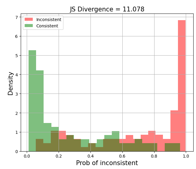 Separation of distributions with JS divergence = 11.078 (View Highlight)
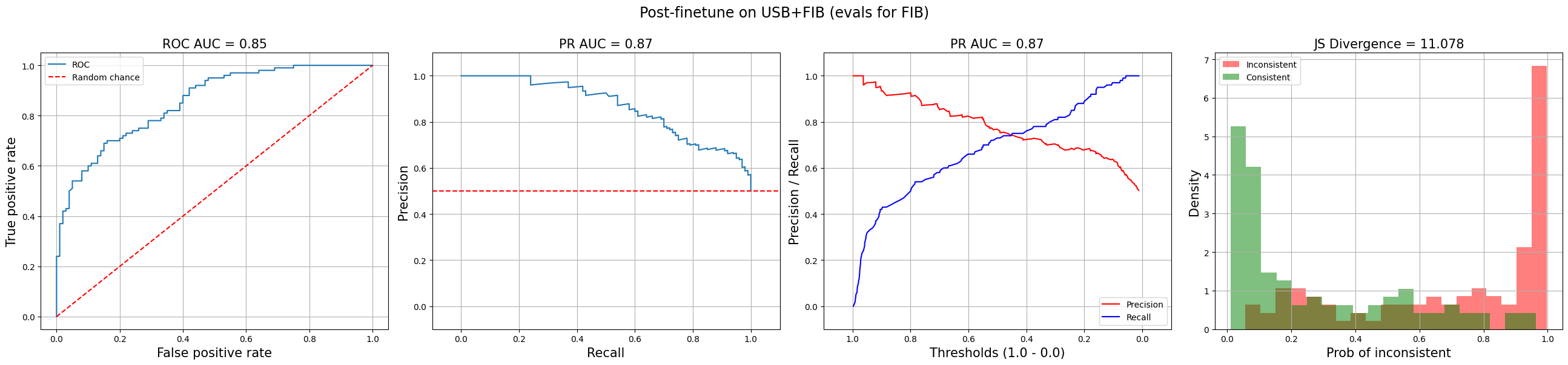 Diagnostic plots for classification tasks (View Highlight)