Customer lifetime value (CLV) is a crucial metric to evaluate and steer long-term success for a product or service. We not only want to optimize the cost per-cost per acquisition (for example, with a media mix model with PyMC-Marketing), but also make sure this investment pays off through long-term revenue generated by users. Many CLV models exist in the literature (for contractual and non-contractual settings). Peter Fader and Bruce Hardie pioneered many of them, especially for models specified through a transparent probabilistic data-generating process driven by the user behavior mechanism. Currently, PyMC-Marketing ‘s CLV module provides the best Python production-ready implementations of these models. Many of these models allow user-level external time-invariant covariates (e.g. acquisition channel) to explain the variance of the data better. (View Highlight)
In strategic business situations, we often need to look beyond user-level CLV and focus on a higher granularity: a cohort. These cohorts can be defined by registration or by first-time date. There are several reasons for working at the cohort level. For one, new privacy regulations such as GDPR might prohibit using sensitive individual-level data in models. In reality, individual-level predictions are not always necessary for strategic decision-making. On the other hand, from a technical perspective, while we can aggregate individual-level CLV at the cohort level, incorporating time-sensitive factors into these models is not straightforward and requires significant effort. (View Highlight)
These observations led to the development of an alternative top-down modeling approach, where we model all cohorts simultaneously. This simple and flexible approach provides a robust baseline for CLV across the entire user pool. The key idea is to combine two model components in a single model: retention and revenue. We can use this model for inference (say, what drives retention and revenue changes) and forecasting. (View Highlight)
We can define the observed retention for a given cohort and period combination as n_active_users / n_users. As this is a synthetic dataset, we have the actual retention values, which we use for model evaluation. (View Highlight)
Next, let’s think about retention as a metric. First, it is always between zero and one; this provides a hint for the likelihood function to choose. Second, it is a quotient. This fact is essential to understanding the uncertainty around it. For example, for cohort A, you have a retention of 20 % coming from a cohort of size 10. This retention value indicates that two users were active out of these 10. Now consider cohort B, which also has a 20% retention but with one million users. Both cohorts have retention, but intuitively, you are more confident about this value for the bigger cohort. This observation hints that we should not model retention directly but rather the number of active users. We can then see retention as a latent variable . (View Highlight)
For this synthetic data set, the model above works well. Nevertheless, disentangling the relationship between features in many real applications is not straightforward and often requires an iterative feature engineering process. An alternative is to use a model that can reveal these non-trivial feature interactions for us while keeping the model interpretable. Given the vast success in machine learning applications, a natural candidate is tree ensembles. Their Bayesian version is known as BART (Bayesian Additive Regression Trees), a non-parametric model consisting of a sum of m regression trees. (View Highlight)
One of the reason BART is Bayesian is the use of priors over the regression trees. The priors are defined in such a way that they favor shallow trees with leaf values close to zero. A key idea is that a single BART-tree is not very good at fitting the data but when we sum many of these trees we get a good and flexible approximation. (View Highlight)
Luckily, a PyMC version is available PyMC BART, which we can use to replace the linear model component from the baseline model above. Concretely, the BART model enters the equation as (View Highlight)
Remark: The response="mix" option in the BART class allows us to combine two ways of generating prediction from the trees: (1) taking the mean and (2) using a linear model. Having a linear model component on the leaves will allow us to generate better out-of-sample predictions. (View Highlight)
As expected from the modeling approach, the credible intervals are wider for the smaller (in this example, the younger) cohorts. (View Highlight)
The out-of-sample predictions are good! The model can capture the trends and seasonal components. (View Highlight)
The PyMC BART implementation provides excellent tools to interpret how the model generates predictions. One of them is partial dependence plots (PDP). These plots provide a way of understanding how a feature affects the predictions by averaging the marginal effect over the whole data set. Let us take a look at how these look for this example: (View Highlight)
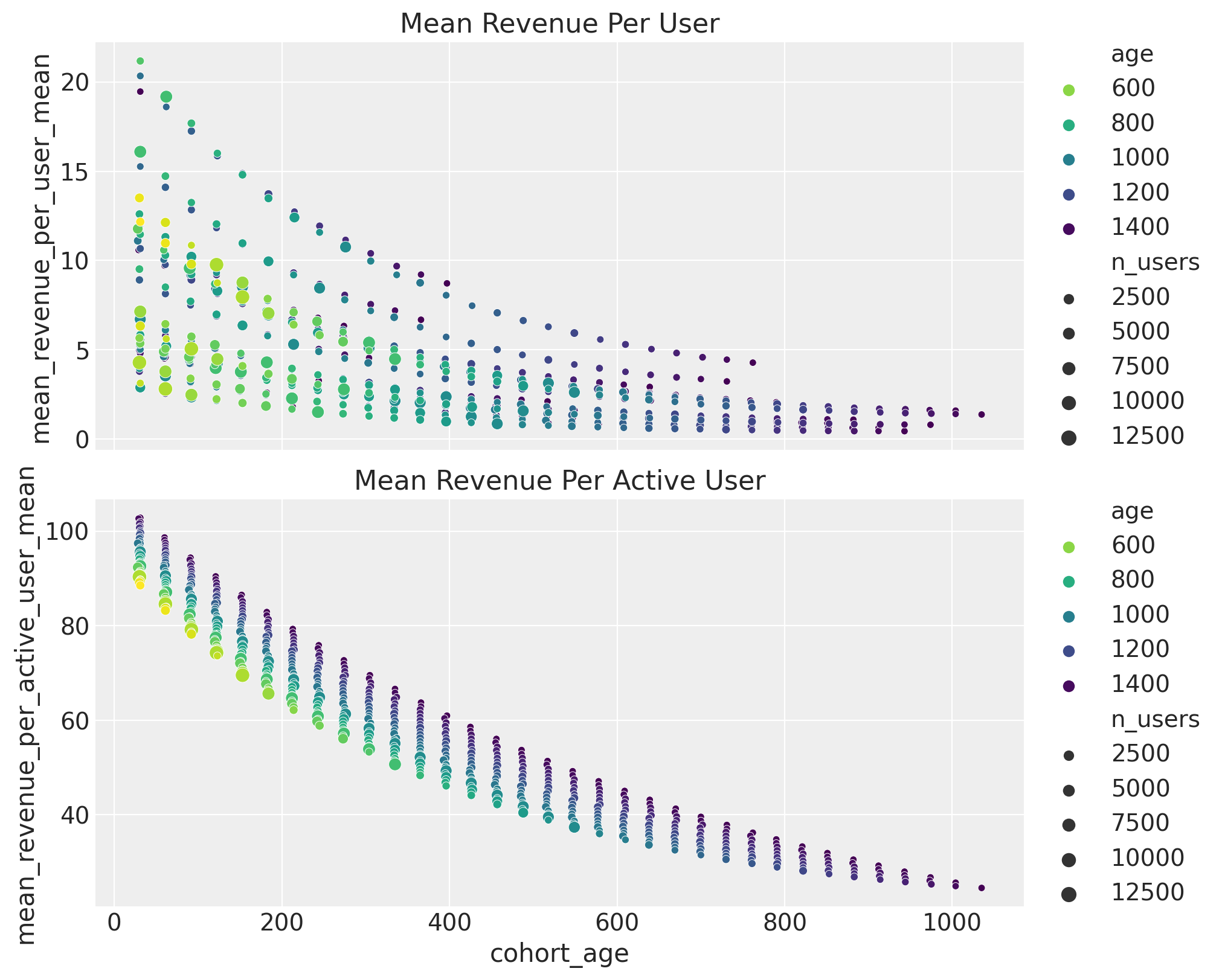
The BART model performs very well on the retention component. Still, our ultimate goal is to predict future cohort-level value measured in money (not just retention metrics). Hence, it is crucial to add the monetary value to the analysis. Fortunately, the Bayesian framework allows enough flexibility to do this in a single model! Let’s think about the revenue variable: (View Highlight)
We can also get insights into the average revenue per user and active user behavior as a function of the cohort features.
(View Highlight)
Another exciting application of this model is causal analysis. For example, assume we ran a global marketing campaign to increase the order rate (for example). Suppose we can not do an A/B test and have to rely on quasi-experimental methods like “causal impact”. In that case, we might underestimate the campaign’s effect if we aggregate all the cohorts together. An alternative is to use this cohort model to estimate the “what-if-we-had-no-campaign” counterfactual at the cohort level. It might be that newer cohorts were more sensitive to the campaign than older ones, and this could explain why we are not seeing a significant effect on the aggregation. (View Highlight)
There are still many things to discover and explore about these cohort-level models. For example, a hierarchical model across markets on which we pool information across many of these retention and revenue matrices. This approach would allow us to tackle the cold-start problem when we do not have historical data. Stay tuned! (View Highlight)

 (View Highlight)