Metadata
- Author: Avi Chawla
- Full Title: MLE vs. EM — What’s the Difference?
- URL: https://www.blog.dailydoseofds.com/p/mle-vs-em-whats-the-difference
Highlights
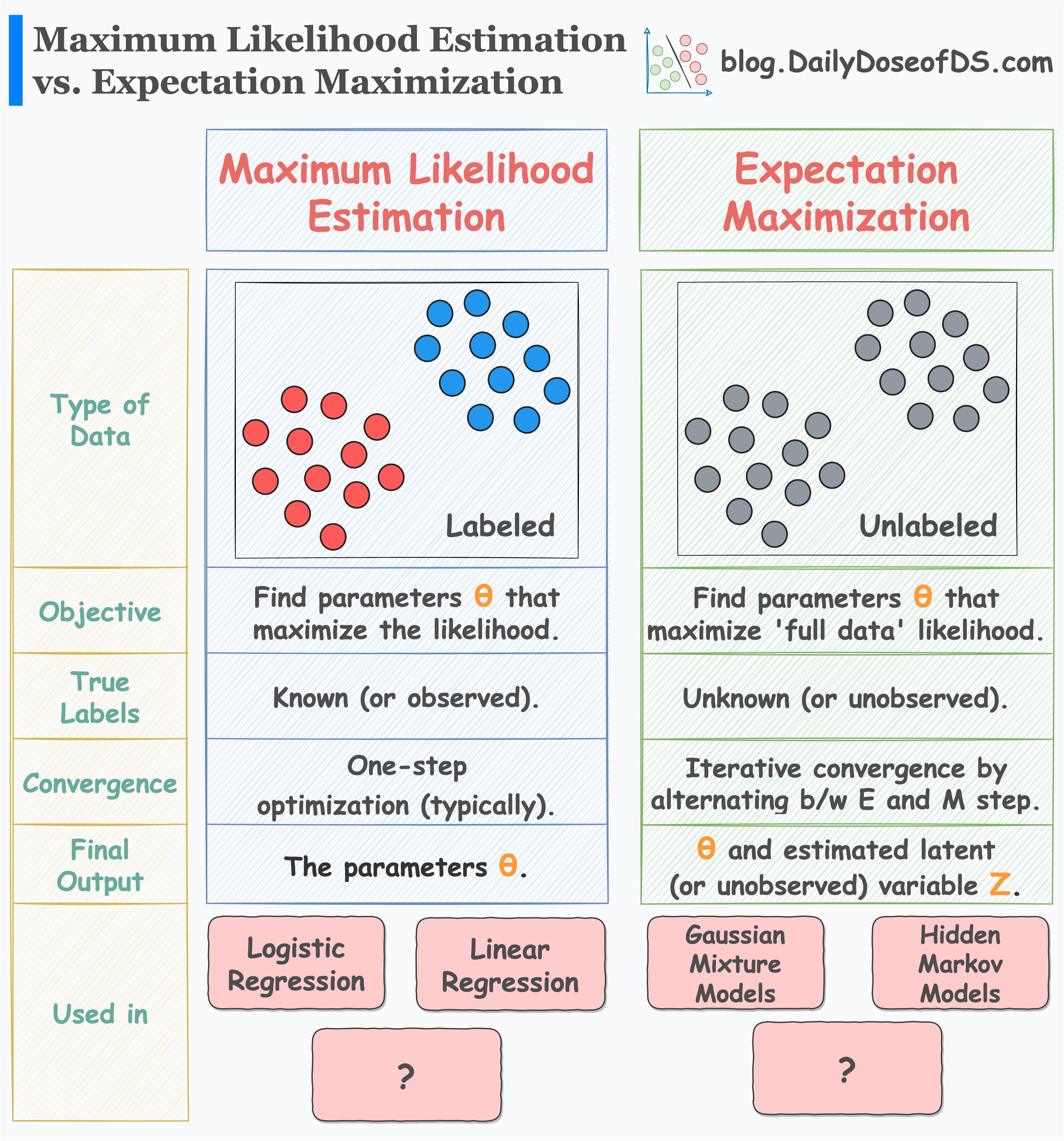
- MLE starts with a labeled dataset and aims to determine the parameters of the statistical model we are trying to fit. (View Highlight)
- Start by assuming a data generation process. Simply put, this data generation process reflects our belief about the distribution of the output label (
y), given the input (X). (View Highlight) - Next, we define the likelihood of observing the data. As each observation is independent, the likelihood of observing the entire data is the same as the product of observing individual observations: (View Highlight)
- Tags: favorite
- The likelihood function above depends on parameter values (θ). Our objective is to determine those specific parameter values that maximize the likelihood function. We do this as follows: (View Highlight)
- EM is an iterative optimization technique to estimate the parameters of statistical models. It is particularly useful when we have an unobserved (or hidden) label. (View Highlight)
- As depicted above, we assume that the data was generated from multiple distributions (a mixture). However, the observed/complete data does not contain that information. (View Highlight)
- In other words, the observed dataset does not have information about whether a specific row was generated from distribution 1 or distribution 2. (View Highlight)
- follows:
• Make a guess about the initial parameters (θ).
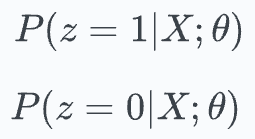
• Expectation (E) step: Compute the posterior probabilities of the unobserved label (let’s call it ‘
z’) using the above parameters. (View Highlight)
 - Maximization (M) step: So now we have a likelihood function to work with. Maximizing it with respect to the parameters will give us a new estimate for the parameters (θ`). (View Highlight)
- The point is that in expectation maximization, we repeatedly iterate between the E and the M steps until the parameters converge. (View Highlight)
 (View Highlight)
 (View Highlight)